- Published on
MLOps Basics [Week 1]: Model Monitoring - Weights and Bias
- Authors

- Name
- Raviraja Ganta
- @raviraja_ganta
📊 ML Model Monitoring
Why should you monitor your model? There are many reasons. It can help you understand the accuracy of your predictions, prevent prediction errors, and tweak your models to perfect them.
Generally we will be running experiments by tweaking hyper-parameters, trying different models to test their performance, see the connection between your model and the input data, and perform advanced tests. Having all these logged at a single place will help in getting better and faster insights.
The easiest way to ensure things work smoothly is to use ML model monitoring tools.
Dedicated tools can also be used to collaborate with your team, share your work with other people—it’s a shared space for teams to collaborate, participate in model creation and further monitoring. It’s easier to exchange ideas, thoughts and observations, and spot errors when you have real-time insight into what’s happening with your models.
There are many libraries available to monitor machine learning models. The prominent ones are:
and many more...
I will be using Weights and Bias.
In this post, I will be going through the following topics:
How to configure basic logging with W&B?How to compute metrics and log them in W&B?How to add plots in W&B?How to add data samples to W&B?
Note: Basic knowledge of Machine Learning, Pytorch Lightning is needed
🏋️ Weights and Bias Configuration
In order to use W&B, an account needs to be created. (Free for public projects and 100GB storage). Once account is created, we need to login.
Run the command:
wandb login
You will be prompted with the following:


Follow the authorisation link: https://wandb.ai/authorize and copy paste the api key.
Configuring 🏋️ 🤝 ⚡️
Create a project at W&B and then use the same name here. So that all the experiments will be logged into that project.
from pytorch_lightning.loggers import WandbLogger
wandb_logger = WandbLogger(project="MLOps Basics")
Now pass this as the logger to the Trainer.
trainer = pl.Trainer(
        max_epochs=3,
        logger=wandb_logger,
        callbacks=[checkpoint_callback],
    )
Now all the logs will be tracked in W&B.
📈 Metrics
Metrics calculation can sometimes become daunting. Fortunately pytorch lightning team has been building a library torchmetrics which contains all the prominent metrics. Check the documentation for more information.
Since the problem is about classification, Let's see how to calculate metrics like Accuracy, Precision, Recall, F1.
Let's import the torchmetrics library as
import torchmetrics
Then declare the metrics in __init__
class ColaModel(pl.LightningModule):
    def __init__(self, model_name="google/bert_uncased_L-2_H-128_A-2", lr=3e-5):
        self.train_accuracy_metric = torchmetrics.Accuracy()
        self.val_accuracy_metric = torchmetrics.Accuracy()
        self.f1_metric = torchmetrics.F1(num_classes=self.num_classes)
        self.precision_macro_metric = torchmetrics.Precision(
            average="macro", num_classes=self.num_classes
        )
        self.recall_macro_metric = torchmetrics.Recall(
            average="macro", num_classes=self.num_classes
        )
        self.precision_micro_metric = torchmetrics.Precision(average="micro")
        self.recall_micro_metric = torchmetrics.Recall(average="micro")
Metrics can be calculated at different steps like during training, validation and testing.
Pytorch Lightning Module ⚡️ comes with different methods which makes our job easy on where to implement the metrics calculation.
The two main methods where the metrics usually calculated are:
training_step: This is where a batch of training data is processed. Metrics liketraining loss,training_accuracycan be computed here.validation_step: This is where a batch of validation data is processed. Metrics likevalidation_loss,validation_accuracyetc can be computed here.
There are other methods also available:
training_epoch_end: This is called at the end of every training epoch. All the data which is returned bytraining_stepcan be aggregated here.validation_epoch_end: This is called at the end of every training epoch. All the data which is returned bytraining_stepcan be aggregated here.test_step: This is called when trainer is called with test method i.etrainer.test().test_epoch_end: This is called at the end of all test batches.
Few configurations available for logging:
- Setting
prog_bar=Truewhich will enable to show metrics on the progress bar. - Setting
on_epoch=True, the metrics will be aggregated and averaged across the batches in an epoch. - Setting
on_step=True, the metrics will be logged for each batch. (useful for loss)
By default:
- Logging in
training_stephason_step=True - Logging in
validation_stephason_step=False,on_epoch=True
For more, refer to the documentation here
Now let's see how metrics calculation and logging looks like:
def training_step(self, batch, batch_idx):
outputs = self.forward(
batch["input_ids"], batch["attention_mask"], labels=batch["label"]
)
# loss = F.cross_entropy(logits, batch["label"])
preds = torch.argmax(outputs.logits, 1)
train_acc = self.train_accuracy_metric(preds, batch["label"])
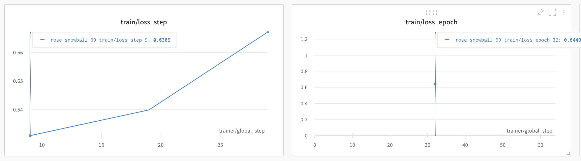
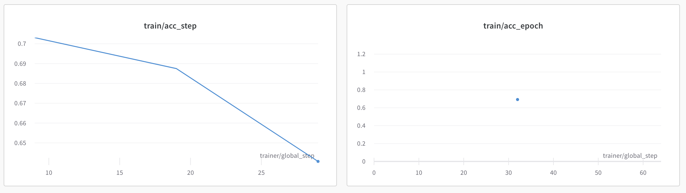
self.log("train/loss", outputs.loss, prog_bar=True, on_epoch=True)
self.log("train/acc", train_acc, prog_bar=True, on_epoch=True)
return outputs.loss
Since on_epoch=True is enabled, the plots in W&B 🏋️ will have train/loss_step, train/loss_epoch and train/acc_step, train/acc_epoch.


During validation, we might want to monitor more metrics like Precision, Recall, F1.
def validation_step(self, batch, batch_idx):
labels = batch["label"]
outputs = self.forward(
batch["input_ids"], batch["attention_mask"], labels=batch["label"]
)
preds = torch.argmax(outputs.logits, 1)
# Metrics
valid_acc = self.val_accuracy_metric(preds, labels)
precision_macro = self.precision_macro_metric(preds, labels)
recall_macro = self.recall_macro_metric(preds, labels)
precision_micro = self.precision_micro_metric(preds, labels)
recall_micro = self.recall_micro_metric(preds, labels)
f1 = self.f1_metric(preds, labels)
# Logging metrics
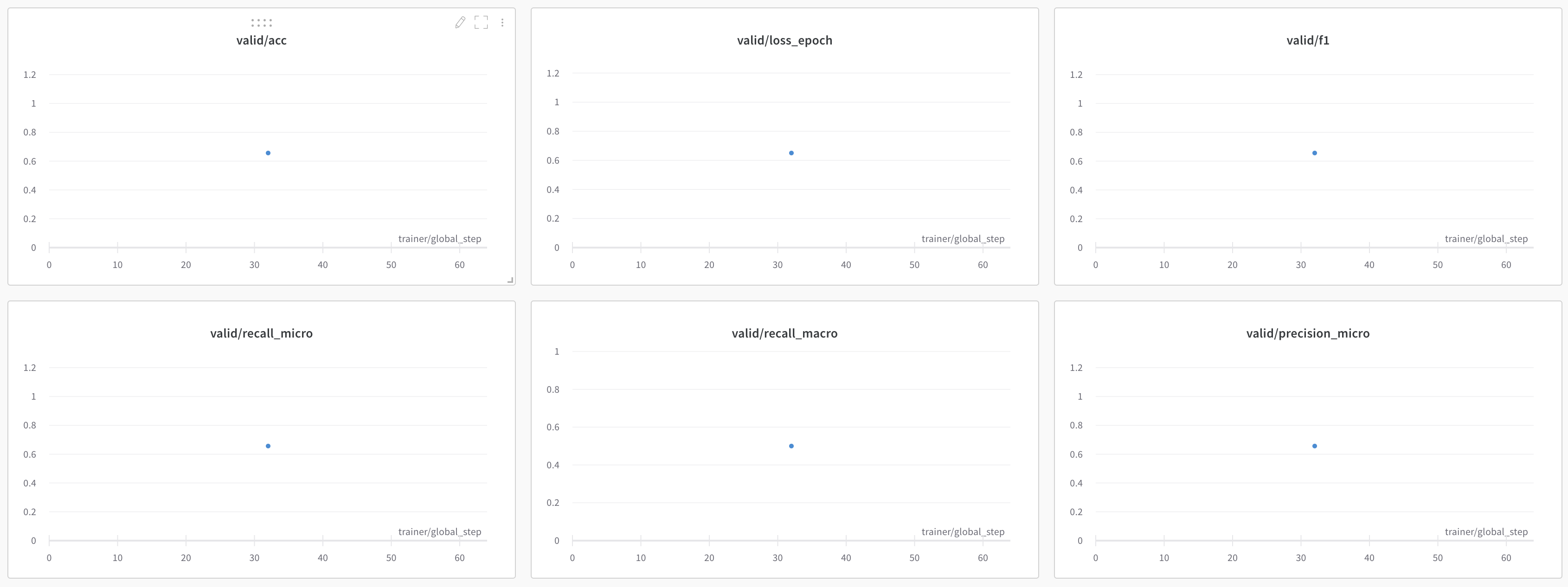
self.log("valid/loss", outputs.loss, prog_bar=True, on_step=True)
self.log("valid/acc", valid_acc, prog_bar=True)
self.log("valid/precision_macro", precision_macro, prog_bar=True)
self.log("valid/recall_macro", recall_macro, prog_bar=True)
self.log("valid/precision_micro", precision_micro, prog_bar=True)
self.log("valid/recall_micro", recall_micro, prog_bar=True)
self.log("valid/f1", f1, prog_bar=True)
return {"labels": labels, "logits": outputs.logits}

The values returned during the validation_step can be aggregated in the validation_epoch_end and any transformations can be done using that.
For example, as shown in the above code snippet labels, logits are returned.
These values can be aggregated in the validation_epoch_end method and metric like confusion matrix can be computed.
def validation_epoch_end(self, outputs):
    labels = torch.cat([x["labels"] for x in outputs])
    logits = torch.cat([x["logits"] for x in outputs])
    preds = torch.argmax(logits, 1)

    cm = confusion_matrix(labels.numpy(), preds.numpy())
📉 Adding Plots to 🏋️
Logging metrics might not be sufficient every time. Having more visual information like graphs and plots will help in understanding the model performance better.
There are multiple ways to plot graphs in 🏋️. Let's see a couple of ways.
As an example, let's see how to plot confusion_matrix computed above.
Method 1
🏋️ has built-in wandb.plot methods (preferrable since it offers lot of customizations). Check for all available methods here: documentation
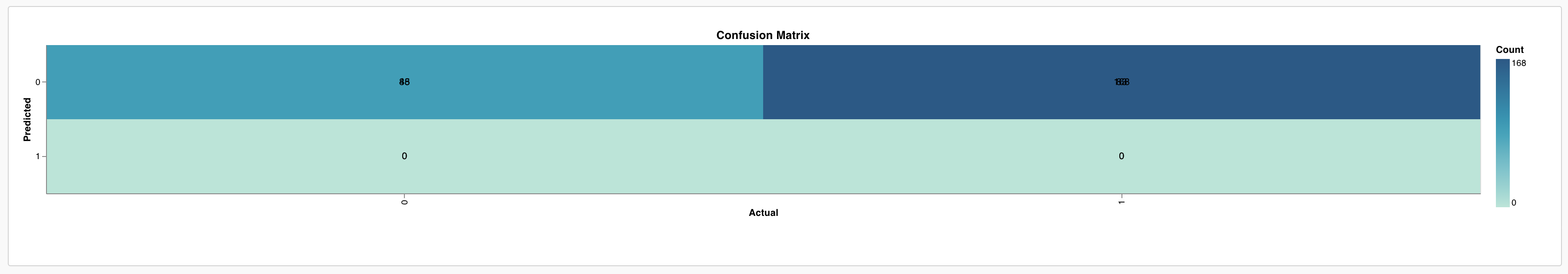
Plotting confusion matrix looks like:
# 1. Confusion matrix plotting using inbuilt W&B method
self.logger.experiment.log(
    {
        "conf": wandb.plot.confusion_matrix(
            probs=logits.numpy(), y_true=labels.numpy()
        )
    }
)
The plot looks like:

Method 2
🏋️ supports scikit-learn integration also. Which means whatever the plots available in scikit-learn can be plotted in 🏋️. Refer to the documentation for more details.
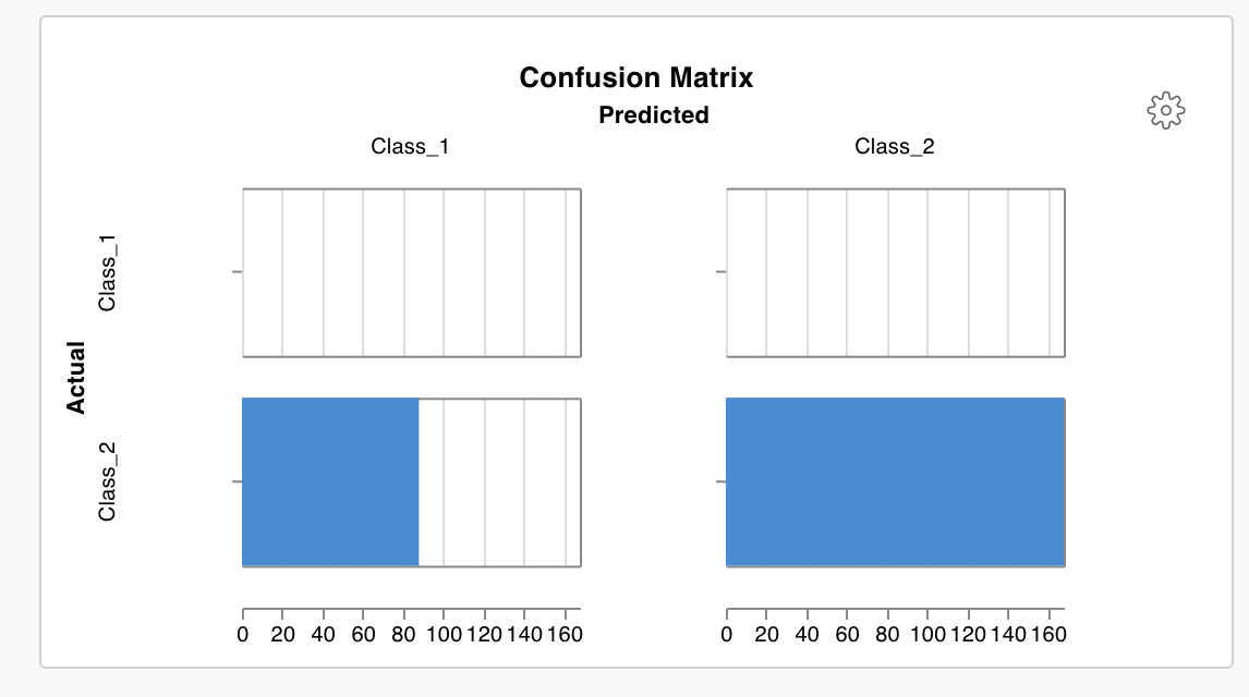
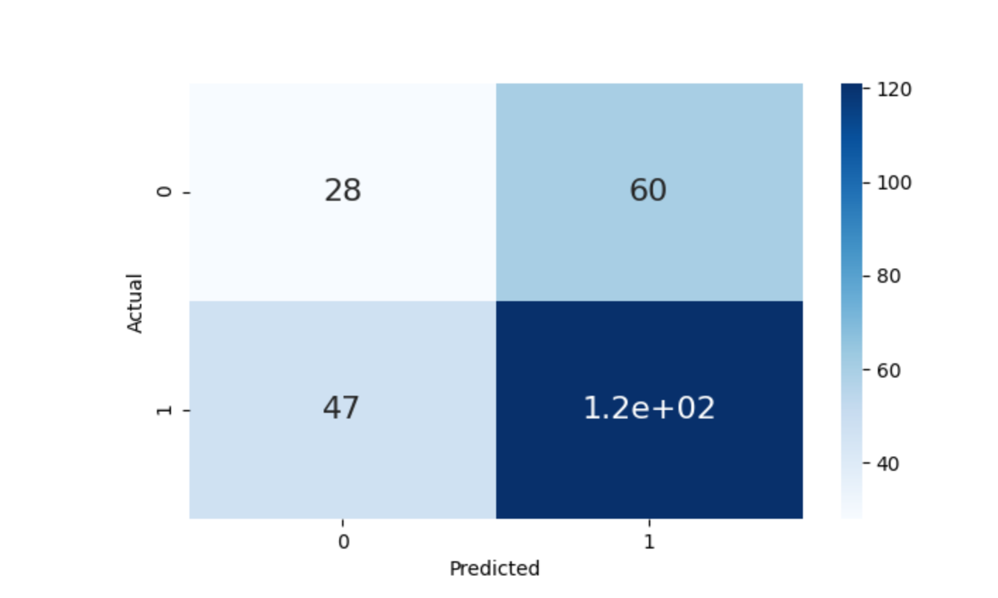
Plotting of confusion matrix using scikit-learn looks like:
# 2. Confusion Matrix plotting using scikit-learn method
wandb.log({"cm": wandb.sklearn.plot_confusion_matrix(labels.numpy(), preds)})
The plot looks like:

Method 3
🏋️ supports plotting libraries matplotlib, plotly etc. Refer to the documentation for more details.
This means we can create our own plot and log them in 🏋️
# 3. Confusion Matric plotting using Seaborn
data = confusion_matrix(labels.numpy(), preds.numpy())
df_cm = pd.DataFrame(data, columns=np.unique(labels), index=np.unique(labels))
df_cm.index.name = "Actual"
df_cm.columns.name = "Predicted"
plt.figure(figsize=(10, 5))
plot = sns.heatmap(
    df_cm, cmap="Blues", annot=True, annot_kws={"size": 16}
)  # font size
self.logger.experiment.log({"Confusion Matrix": wandb.Image(plot)})
The plot looks like:

Now that we know how to add graphs in 🏋️ , let's see how to add data samples (images, text etc) to 🏋️
📝 Adding Data samples to 🏋️
Once the model is trained, we need to understand where the model is performing well and where it is not.
Since we are working on cola problem, let's look at few samples where the model is not performing good and log it to 🏋️
There can be a lot of ways to plot the data. Refer to documentation here for more details.
This can be achieved via callback 🔁 mechanism in ⚡️
class SamplesVisualisationLogger(pl.Callback):
    def __init__(self, datamodule):
        super().__init__()

        self.datamodule = datamodule

    def on_validation_end(self, trainer, pl_module):
        # can be done on complete dataset also
        val_batch = next(iter(self.datamodule.val_dataloader()))
        sentences = val_batch["sentence"]

        # get the predictions
        outputs = pl_module(val_batch["input_ids"], val_batch["attention_mask"])
        preds = torch.argmax(outputs.logits, 1)
        labels = val_batch["label"]

        # predicted and labelled data
        df = pd.DataFrame(
            {"Sentence": sentences, "Label": labels.numpy(), "Predicted": preds.numpy()}
        )

        # wrongly predicted data
        wrong_df = df[df["Label"] != df["Predicted"]]

        # Logging wrongly predicted dataframe as a table
        trainer.logger.experiment.log(
            {
                "examples": wandb.Table(dataframe=wrong_df, allow_mixed_types=True),
                "global_step": trainer.global_step,
            }
        )
Then add this callback 🔁 to trainer 👟
trainer = pl.Trainer(
        max_epochs=3,
        logger=wandb_logger,
        callbacks=[checkpoint_callback, SamplesVisualisationLogger(cola_data)],
        log_every_n_steps=10,
        deterministic=True,
    )
In 🏋️ this will look like

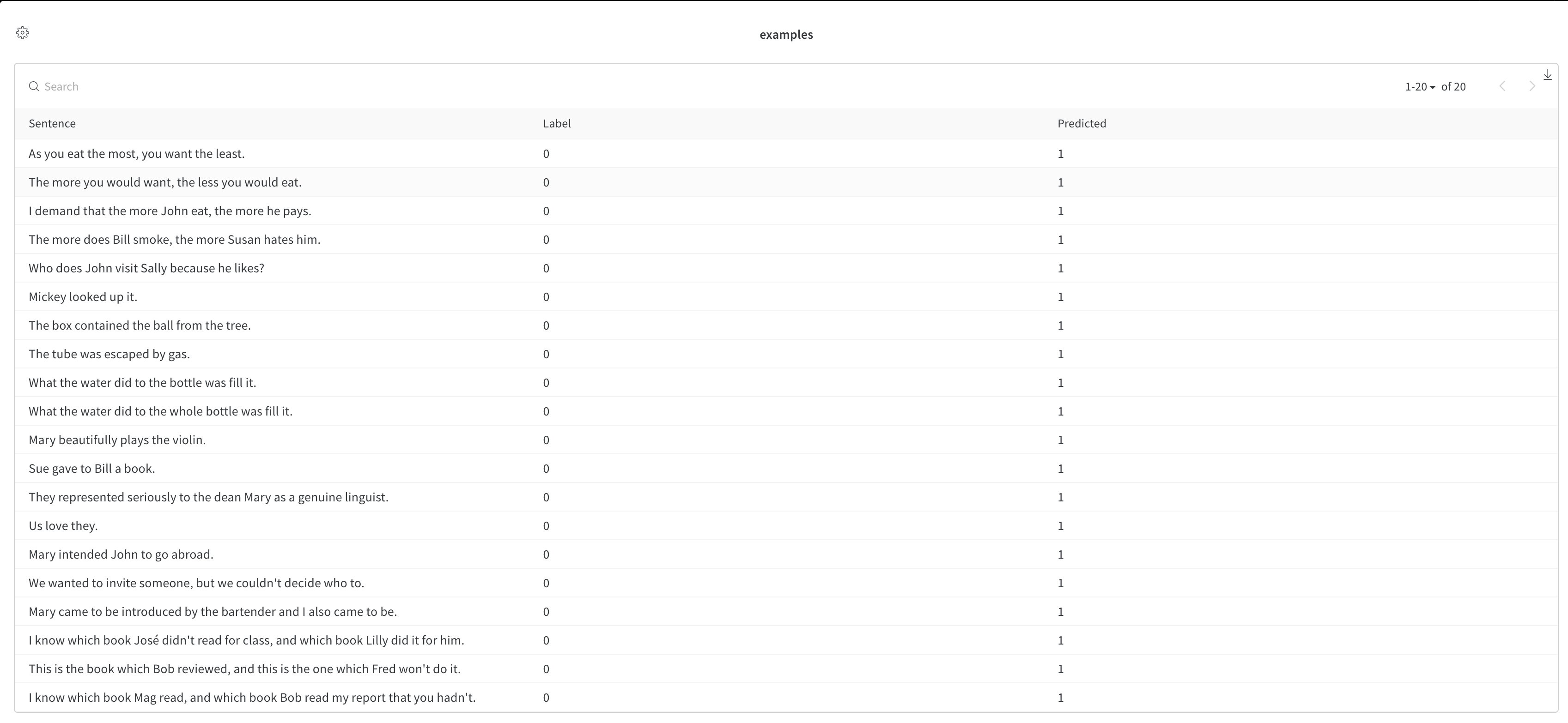
🔚
This conculdes the post. In the next post, I will be going through:
How to do configuration using Hydra?
Complete code for this post can also be found here: Github